Your cart is currently empty!


VLOOKUP is a powerful formula in Google Sheets and Excel that lets you fill a cell with information from another using a lookup key. This guide covers the basics of the VLOOKUP function and how to use it in your spreadsheets.
VLOOKUP Basics
The formula for VLOOKUP in Google Sheets looks like this:
Formula Syntax
=VLOOKUP(search_key, range, index, [is_sorted])Input Details
- search_key: What you’ll use to search for other data.
- range: The range of data you want searched.
- index: What column in the range you want.
- is_sorted: Binary value for indicating if the data you’re searching is sorted.
Formula Example
Here’s a sample VLOOKUP function:
=VLOOKUP(D2,A2:B10,2,FALSE)Let’s break it down from there.
=VLOOKUP(– Initializing the formula. The “(” signals what will be included.D2– We’re going to “look up” information about this cell. If we were performing keyword research, this might be a keyword.A2:B10– The range of data you want VLOOKUP to search through. Can be a selection, rows from another tab, or whatever you specify.2– Tells the function to look up data from the second column in the range. Here, this indicates we want a value from column B.FALSE– Signaling the data is not sorted; use exact match for the search. Often the first value to mess with if the formula output doesn’t seem right.)– Closes the formula.
This will extract information from cells A2:B10, using D2 as the search key. It will pull the value from the second column of the data range, column B. It will return the value of that cell in place of the formula.
Theory! All well and good, but kinda hard to understand, right? Let’s go through a practical situation for using this in SEO work and content management.
How to Use VLOOKUP
For this tutorial, we’ll use a basic Google Sheets content calendar setup. We’ll walk through a helpful trick for managing keyword data in the sheet VLOOKUP.
Example Result
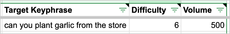
Pull keyword data like search volume from a different spreadsheet tab, using the primary keyword as the lookup key. That might look something like this, where Difficulty and Volume use VLOOKUP values:
The Process
Now, let’s go through how to create a formula like this in Google Sheets.
1. Double-click a cell where you want to return the looked-up value.
2. Type “=vl” and it should show the function.
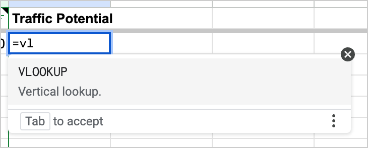
3. Hit Tab to begin the formula. It should change to this:
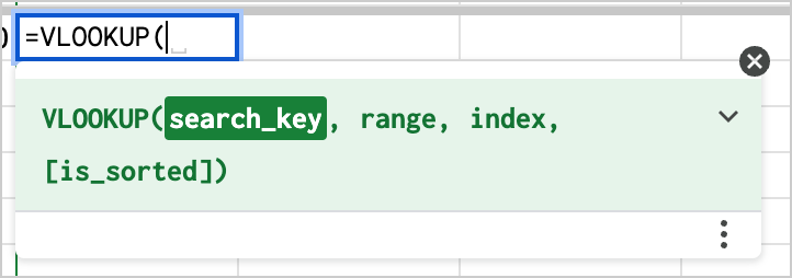
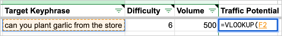
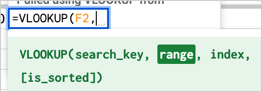
4. Click on the cell you want to use as the search key. In our case, this is F2, the cell in the Target Keyphrase column.
5. Add a comma to the formula. This prepares the function so you can select the range.
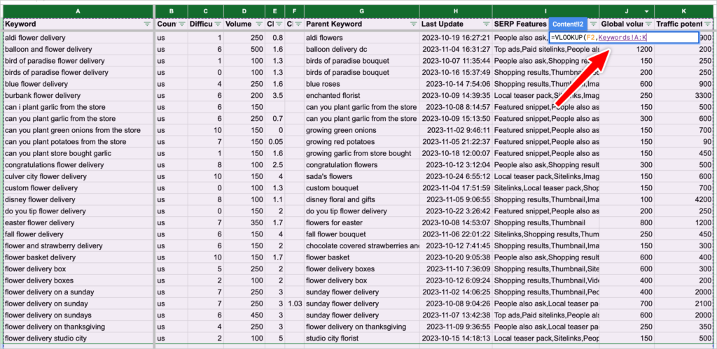
6. Select the cells you want to search. This will vary depending on your situation.
In our case, we want to select the columns in the Keywords tab, so we’ll click the Keywords tab, then click-drag across the active columns to select the range:
7. Add another comma to proceed and prepare for the index value.
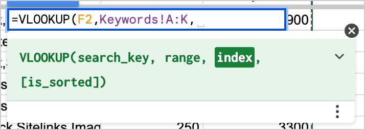
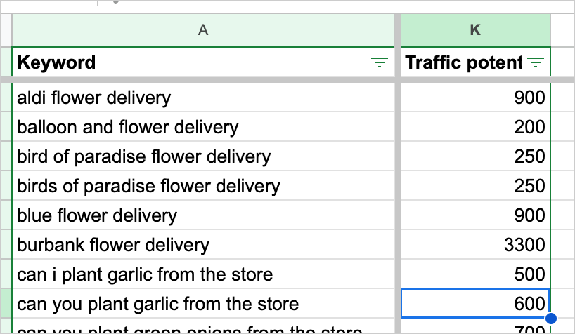
8. Enter the column number you want to reference from your range. VLOOKUP needs to know what “index” it should pull from in your selected range.
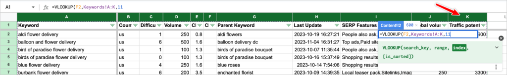
In our case, that number is 11 because K is the 11th column in the selection from A-K. If you wanted to look up a different value like “Volume”, you’d enter “4”.
9. Add a comma. The final one! Technically, the next field is optional, but it’s best to be explicit when filling out the formula.
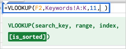
10. Type zero “0” or another false value like “FALSE” to indicate the range is not sorted.
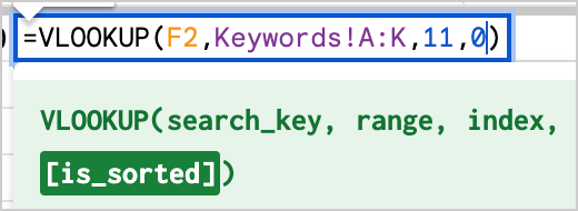
11. Finally, press Enter to run the function.
Final Result
This should update the cell’s value to what you specified in the formula:
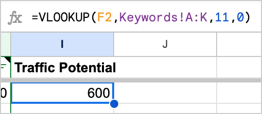
In our example, VLOOKUP returns a value of 600, which is the keyword’s traffic potential value in the keywords tab:
If all goes well, you should see similar results. If not…
Troubleshooting
Don’t worry if the formula doesn’t behave right on your first try. Here are some common issues when using VLOOKUP:
- Incorrect use of TRUE or FALSE for the
[is_sorted]argument. - The lookup value isn’t in the first column of your range.
- Mismatched data types (e.g., looking up a number against text).
For more information, see Google’s official documentation and other online resources.
Bottom Line
VLOOKUP is a powerful formula, but it can be tricky to master. Try it with some practice data and see what you can do. Keep at it until you understand the function and how to use each input. Then, you can save gigantic amounts of time in Google Sheets.
Topics